Plant material and growing conditions
Three medicinal cannabis genotypes provided by Cann Group Ltd (https://www.canngrouplimited.com/, accessed on 22/03/2024) were employed in this study. These genotypes included one high CBDA strain, “Cannatonic,” and two high THCA strains, “Hindu Kush” and “Northern Lights” (previously referred to as “CBD1,” “THC6,” and “THC1,” respectively)42. These genotypes had also been previously used in the same growth system in our study on photoperiod responses25. These lines were initially chosen because they were all popular medicinal cannabis cultivars but phenotypically and genetically distinct, thus provided information directly relevant to the industry while also providing an indication of the genotype-specificity of observed responses.
All plants were cultivated in a secure facility approved by the Australian Government Department of Health and Aged Care Office of Drug Control (ODC). The experiments were carried out under a Commonwealth license and associated permits. Temperature and humidity were maintained at 25 °C and 50%, respectively. The plants were grown in controlled environments (CE) throughout their life cycle, and they were moved within the CEs on a weekly basis during the flowering period to account for any environmental variations.
The cloning and propagation method used has been previously documented42. Experimental plants were cloned from donor mothers. Approximately 15 cm of new growth stems were excised from the mother plants. All leaves on the stem sides were removed, leaving only the top leaf bunch. The bottom of the stem was cut diagonally across a node, creating a clone approximately 12 cm in height. The top leaf bunch was trimmed to the height of the smallest emerging leaf to reduce water loss and prevent overlapping in the propagation dome. The bottom 1 cm of the stem, where roots would form, was lightly scraped with a scalpel, dipped in hormone gel (Clonex Purple, Yates, DuluxGroup, Clayton, Australia), and placed in an organic propagation cube (Eazyplug CT12, Goirle, The Netherlands, eazyplug.nl).
Once the propagation tray was filled with new clones, it was positioned in a propagation dome (Smart Garden heavy-duty 3-piece propagation kit, Epping Hydroponics) for 14 days. The clones were subjected to an 18-hour light/6-hour dark (18 L:6D) photoperiod in a growth cabinet (Conviron A2000, Conviron Asia Pacific Pty Ltd, Grovedale, Australia) at a light intensity of 100 µmol m² s⁻¹ and a temperature of 25 °C. Humidity was gradually reduced over the 14-day propagation period. Plants with established roots were then transplanted into 1.8-litre pots containing a 30:70% blend of perlite and coco-coir with an electrical conductivity (EC) of < 0.5 mS/cm (Professors Nutrients, Australia). Subsequently, the plants were transferred to controlled flowering environments under a photosynthetically active radiation (PAR) of 600 µmol m² s⁻¹ (Heliospectre Grow Light, LX602C) and maintained under an 18 L:6D photoperiod for an additional 5 days as a hardening period to acclimate to the new environment. After the additional 5 days, the photoperiod was switched to one of the 6 treatments described below and flowering was initiated. The temperature ranged from 20 oC (night) to 26 °C (day), and blackout curtains prevented light leakage. The plants were watered and fed using a commercial fertigation recipe with an electrical conductivity (EC) of 2.2 mS/cm and a pH of 6. As there was an odd number of plants (21) within each treatment, plants were spaced 10 cm apart in 40 × 50 cm grid with an extra plant on the end of the row. As plants were kept small (see Peterswald et al. 2023), this setup assured that plants did not shade each other. To avoid edge effects plant positions were shifted in the chambers twice per week during watering.
Treatments
Each treatment contained 7 replicates of each of the 3 genotypes in a fully randomised design. The six zones were programmed to one of each of the following photoperiods with different timing applications of FR as presented in Table 2. All plants were maintained in these treatments for 40 days, which was the day after cloning (DAC) 70, which is the end point of the flowering treatments.
The 6 programmed zones were controlled using Heliospectre Software (heliospectra.com). A description of each six light spectrum treatments is described in Table 3. The light intensity drops for all treatments from hour 8 because the maximum power (µMol m2 S-1) of the red light band (660 nm) is more powerful than the maximum of the FR band (735 nm) therefore, in order to achieve a low ratio, the FR had to be turned up and the red band down. Treatments not receiving FR in the light period were treated the same to ensure that the daily PAR was consistent between treatments. The height of the plants from the lights was not periodically adjusted because our experiments were designed to represent conditions in commercial facilities in which the bench height and lighting infrastructures are typically fixed. The temperature within the treatments at canopy height was 26 oC under the full spectrum lights and 24 oC under FR only and 20 oC with all lights off.
Measurements
Photosynthetically active radiation (PAR) and the PAR of blue (460 nm), red (660 nm) and white (5700 K) light was measured using a LightScout Quantum Meter and Far Red (735 nm) was measured using a LightScout Red/Far Red Meter (spec-meters.com)/ (accessed on October 19, 2023).
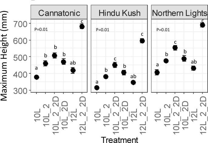
Flowering development was assessed on a weekly basis starting from Day After Cloning 37 (DAC 37) to ascertain the presence or absence of pistils (scored as 1/0) and trichomes (scored as 1/0). Plant height was measured weekly, commencing from DAC 30.
The harvest took place on DAC 70. Plants were excised at the base, and then the whole plant was weighed (whole plant FW). The large fan leaves were removed, and the flowers were manually stripped from the stem and trimmed using a mechanical trimmer (TrimPro ROTOR, Canada). The trimmed flowers were re-weighed (trimmed flower fresh weight) and placed into a foil tray. The flowers were dried in a dedicated drying room at 21 °C and 50% humidity until no further reduction in weight was observed (9 days). The samples were then re-weighed, and the total flower dry weight (g plant− 1) was calculated.
Analytics
The methodology for quantifying cannabinoids has been previously documented28. For each of the 6 treatments and control groups, 4 biological replicates were analyzed for THCA and THC (in the cases of Hindu Kush and Northern Lights) and CBDA and CBD (for Cannatonic), encompassing three different genotypes. Total THC and CBD was then calculated with the following formulae: Total THC = THC + (THCA*0.877) and Total CBD = CBD + (CBDA*0.877).
From each individual plant, three florets were randomly selected from the dried subsample of flower material and finely ground into a powder using liquid nitrogen. A 0.1-gram sub-sample was employed for cannabinoid quantification, which involved sonication in 100% ethanol using a SONICLEAN instrument (Soniclean®, Dudley Park, Australia) operating at 50/60 Hz for 30 min, followed by centrifugation at 10,000 rpm for 10 min. The resulting ethanolic extracts were preserved at -10 °C until needed. Subsequently, these extracts were diluted and subjected to analysis through high-performance liquid chromatography coupled with quadrupole time-of-flight mass spectrometry (UHPLC-QToFMS, Agilent Technologies, Santa Clara, CA, USA). Separation was achieved using a reversed-phase column (Agilent Infinity Poroshell 120, HPH-C18, 2.1 × 150 mm, 2.7 μm, narrow bore LC column, Agilent Technologies, Santa Clara, CA, USA) with mobile phases consisting of methanol-water-acetonitrile and acetonitrile, both containing 0.1% formic acid (v/v). The analysis was executed using Quant Analysis Software 10.2 (Agilent Technologies, Santa Clara, CA, USA), and cannabinoid peaks were identified based on their mass-to-charge (m/z) values and retention times by calibration against cannabinoid standards (Novachem, VIC, Australia).
The total yield of each cannabinoid in g per plant (g plant− 1) was calculated as follows:
((%Cannabinoid/100) x Total flower dry weight in grams) = g cannabinoid plant− 1.
Power use calculations
The kWh used by each of the treatments was calculated using an amp meter (Hioki AC Clamp Meter 3280–10 F, Hioki, Singapore), with a resolution of 0.01 A. The lights were LEDs so there was no “ramp up” or down period and so the amperage requirement for a single setting (e.g. 12 L–2 h of FR in the dark) does not change. At a single timepoint, the amp meter was fitted to each light treatment and the current draw (power drawn from the grid) was recorded. Amps were then converted to kW and multiplied by the photoperiod duration (e.g. 12 h at full spectrum + 2 h of far-red). The carbon emissions per kWh for New South Wales (NSW) Australia were sourced from The Australian Greenhouse Accounts Factors 202229.
Statistical analyses
All graphics and statistical analyses were performed in R 3.143. One way ANOVA’s were performed per variety and Tukey HSD tests were used to identify pair-wise differences between treatments significance for all tests was set at ≤ 0.05. In circumstances were the ANOVA returned a significant statistic but the Tukey HSD test could not identify difference at the ≤ 0.05, a Least Significant Differences (LSD) test was performed using the agricolae package in R43,44.